逻辑回归背后的数学
逻辑回归最先应用于二十世纪早期的生物科学,后用于许多社科应用,当因变量为分类变量时我们往往使用逻辑回归。
举个栗子
预测一封邮件是否包含垃圾信息
预测肿瘤是否致命
考虑到我们需要区分垃圾邮件的场景,如果我们对这个问题使用线性回归,就需要设立一个基于分类的阈值,如果将恶性分类的值给到0.4,阈值设立为0.5,这些数据点被错误归类,将导致严重的后果。
从例子当中,可以推断出线性回归并不适用于分类问题,因为线性回归是没有边界的,所以逻辑回归就应运而生,它们的值被严格限定在0-1范围内。
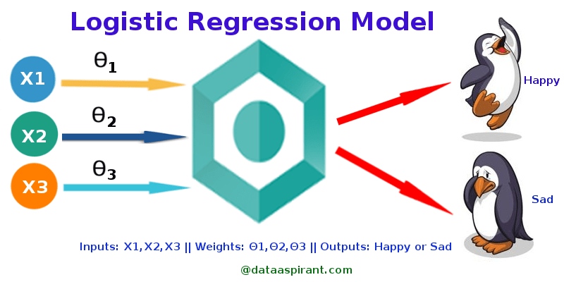
Simple Logistic Regression
Model
1 | Output = 0 or 1 |
Sigmoid Function
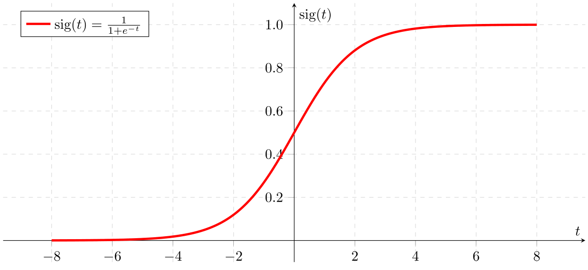
如果Z向无限趋近,则Y值逼近于1,反之为0。
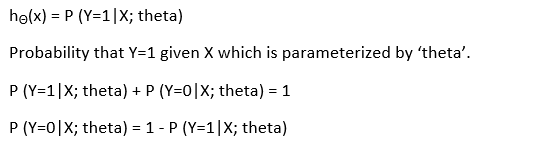
Analysis of the hypothesis
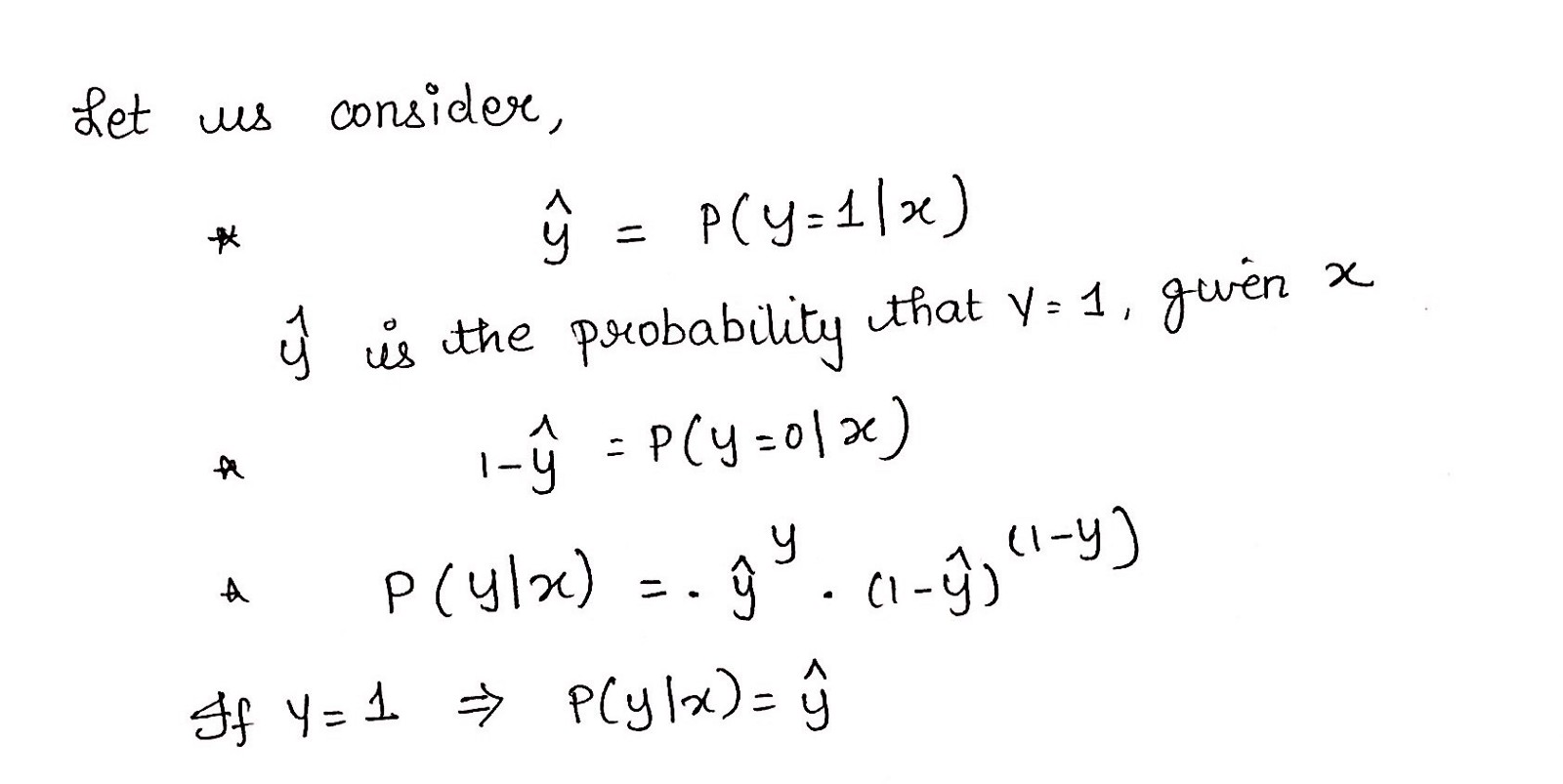
假设的输出结果是估计的概率值。当给定输入X,可以用来推断预测值是实际值的置信度。考虑下面的例子,
1 | X = [x0 x1] = [1 IP-Address] |
基于x1值,假设我们得到的估计概率为0.8。这表明一封电子邮件有80 %的几率是垃圾邮件。
数学公式可以写为:
这证明了“逻辑回归”这个名字的合理性。数据被拟合成线性回归模型,然后由预测目标分类相关变量的逻辑函数对其进行处理。
Types of Logistic Regression
二元逻辑回归
Spam or not多项式逻辑回归
三个甚至多个类型(素食,非素食,肉食)
有序逻辑回归
三个或三个以上有排序的类别。示例:电影等级从1到5
Decision Boundary
为了预测数据的所属分类,需要设立一个阈值,该阈值将得出估计概率的分类类别。
比方说,如果阈值≥0.5,将区分垃圾邮件与否。
决策分解可以是线性或者非线性,而多项式阶数可以增加以获得复杂的决策边界。
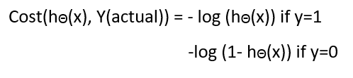
Cost Function
为什么损失函数适用于线性回归而不适用逻辑回归呢?
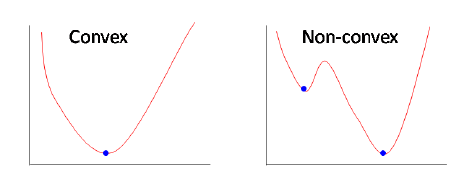
线性回归使用均方误差作为其成本函数。如果这用于逻辑回归,那么它将是参数(θ)的非凸函数。只有当函数是凸的时,梯度下降才会收敛到全局最小值。
like this :)
Cost function explanation
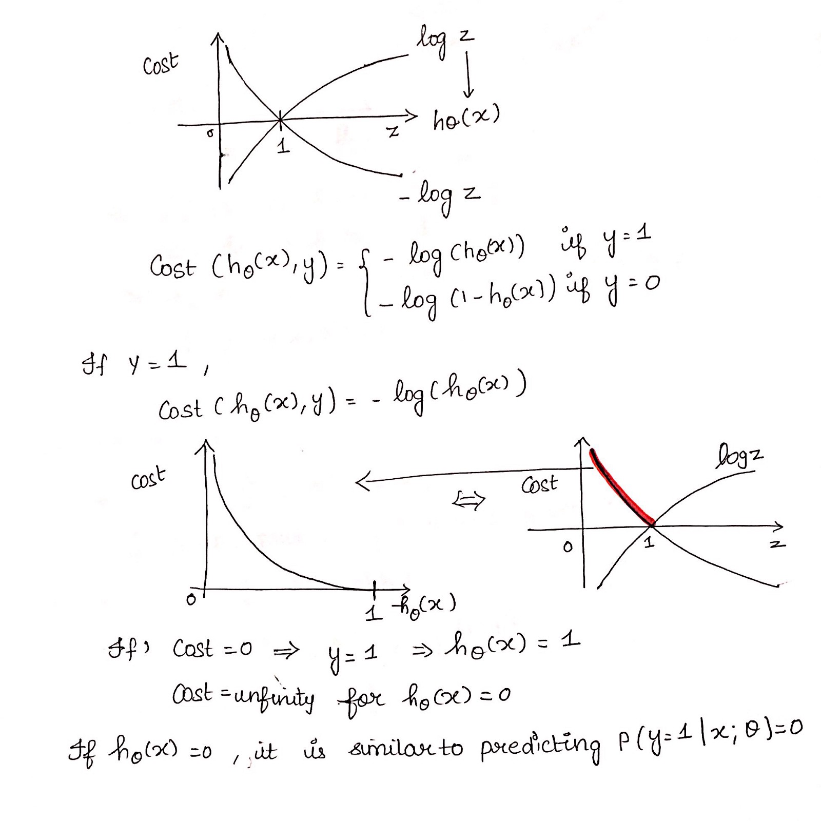
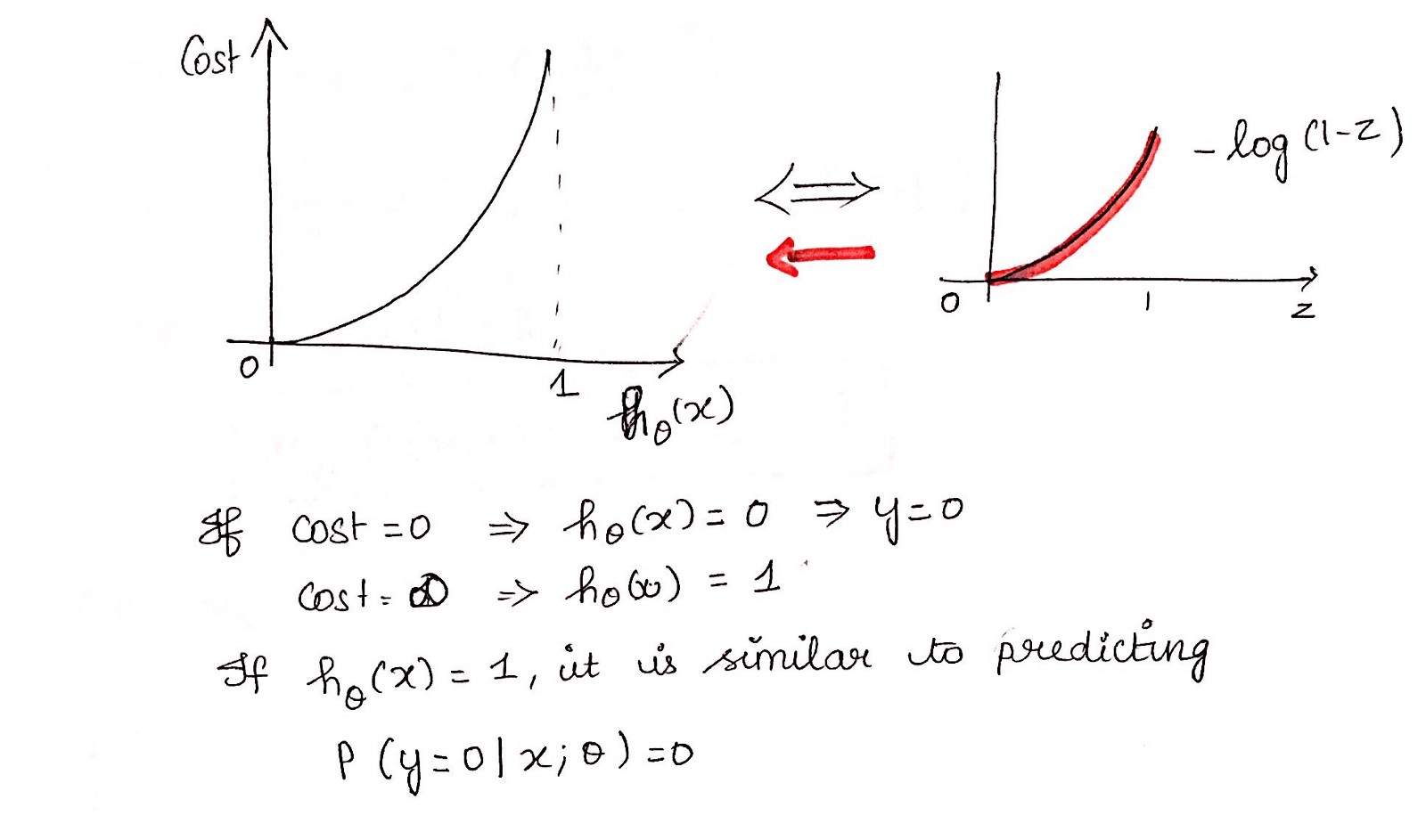
Simplified cost function
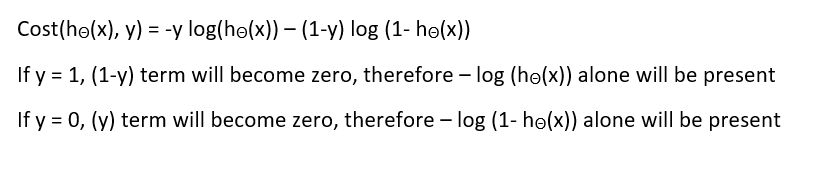
Why this cost function?
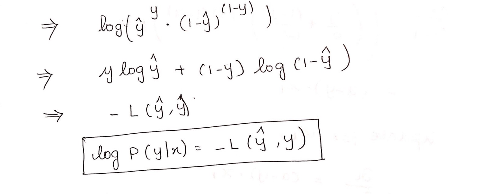
这个负函数是因为当我们训练时,我们需要通过最小化损失函数来最大化概率。假设样本来自相同的独立分布,只有降低成本才能增加最大可能性。
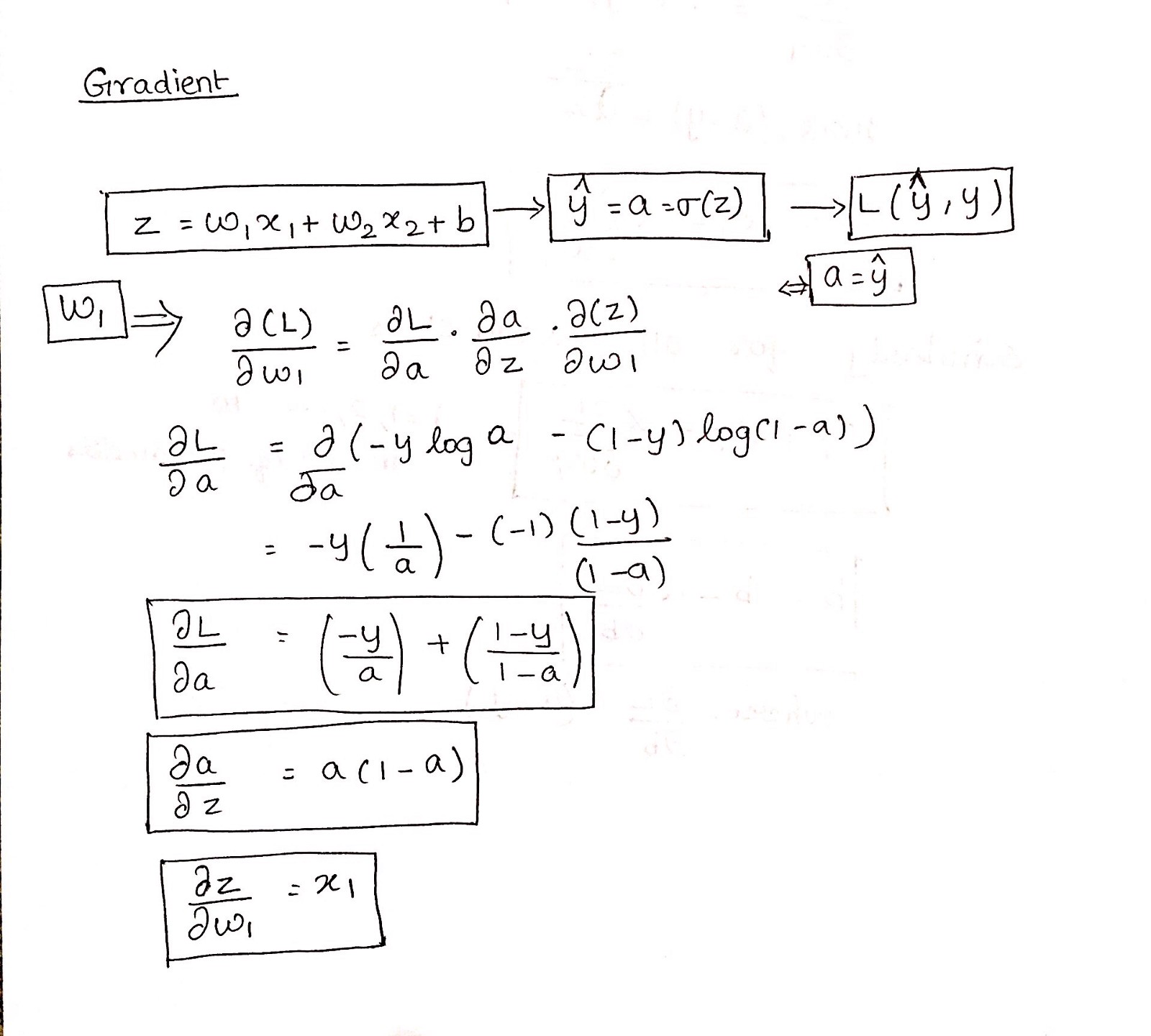
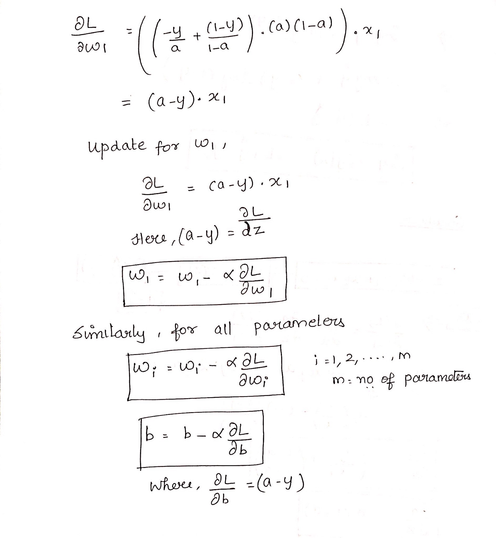
Deriving the formula for Gradient Descent Algorithm
Python Implementation
1 | def weightInitialization(n_features): |
成本与迭代次数的关系:
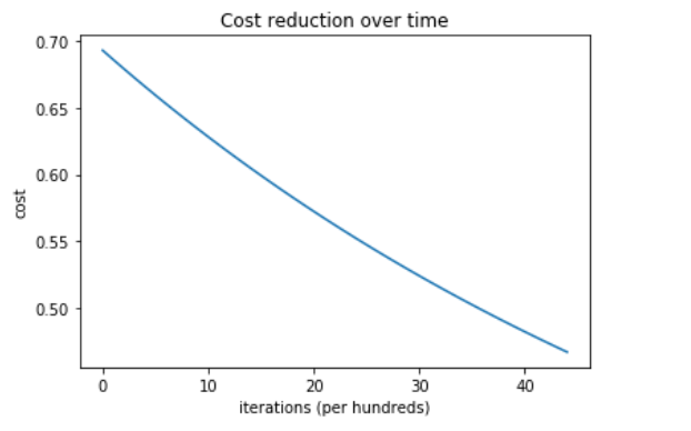
系统的训练和测试精度为100 %
此实现用于二元逻辑回归。对于两个以上类别的数据,必须使用归一化softmax。
原文:https://towardsdatascience.com/logistic-regression-detailed-overview-46c4da4303bc
若你觉得我的文章对你有帮助,欢迎点击上方按钮对我打赏
扫描二维码,分享此文章